First published in May 2021 on SCDA Blog.
One of the duties I frequently performed as an operations research analyst in consulting projects was optimizing companies’ supply chain network designs. A supply chain is a network that connects suppliers with customers to procure materials, transform them into final products, and deliver these products to customers. Supply chain management is a key function of most companies and one of the most exciting management areas. Its goal is to efficiently match supply and demand for final products or services by designing and operating the supply chain. At the strategic level, supply chain design structures the supply chain to strike the right balance between procurement, inventory, transportation, and manufacturing costs as well as the strategic fit. The first step in this process is to determine the supply chain network design, which involves two major decisions:
- Location of sites including production facilities, distribution centers, fulfillment centers, and stores
- Should we add sites to the network?
- Should we shut down existing sites?
- Flow of products
- From where should we source products, and how much should we produce and procure?
- How should we move our products through the network, i.e. which routes and which modes of transport should we use?
These are strategic decisions with significant impact on the company’s cost structure, the resilience as well as the flexibility of the supply chain, and the speed at which products can be shipped to customers. While there is still an inclination to go with the gut when looking at an array of possible supply chain designs, advanced companies understand the value of optimization models to foster a rational decision-making process (see, e.g. Kuttappa, 2020; Gartner, 2019; Burtch Works, 2019; MarketWatch, 2021; Marker, 2017).
There exist an array of technologies for such prescriptive models: open source technologies such as PuLP for Python, SolverStudio for Excel, lpSolve for R, and google’s OR-Tools, as well as powerful commercial technologies such as Gurobi and CPLEX. Additionally, there are vendors offering solutions for common supply chain models, which can potentially increase the productivity to some extent. However, they are less flexible than custom built models and can hence require cumbersome workarounds when there are requirements that are not captured in the standard models.
All network design optimization models are extensions of the well-known facility location problem (or warehouse location problem). Therefore, this post outlines the facility location problem and some scenarios that are typically analyzed during supply chain network design projects. It also elaborates typical ways in which this model is extended to capture requirements of real network design projects.
The facility location problem
I consider the classical facility location problem the simplest supply chain network design model, which is well known in the area of operations research and falls into the category of mixed integer programming models. Simply put, the facility location problem chooses sites from a set of potential sites and determines the flow of product from the chosen sites to customers to satisfy their demands for a single product. Choosing a site incurs fixed cost, and each site has limited capacity. Shipping costs are incurred for the product flow – usually per unit of flow and depending on the distance between origin and destination. The objective is to minimize the total costs.
The customers in this model do not necessarily represent individual end-customers. Instead, they represent markets at a suitable level of aggregation, e.g. countries, states, zip codes, etc. The right level of aggregation depends on the availability of accurate demand data and forecasts. Model complexity may require aggregation too.
In the following example, we consider a retail company based in the USA with customers all across the nation, which currently operates two warehouses located at the east coast. It expects demand to increase in the next five years and considers increasing competitiveness in terms of delivery speeds. Therefore, the company wants to expand its supply chain network. In order to do this in a rational way, it has decided to consult an optimization model.
The baseline scenario
The first major milestone when building an optimization model is always to land the baseline. That baseline considers historical input data and historical decisions. If we then solve the model, we expect the outputs such as total shipping costs to match what we see in the historical data. If there is a mismatch, the model is a poor representation of reality and we need to find the cause.
Let’s say we have determined the inputs needed for the baseline scenario:
- the yearly fixed costs of both existing sites,
- the average shipping cost per kilometer per unit,
- the historical sales volumes by region, and
- the historical shipment volume from each site to each region.
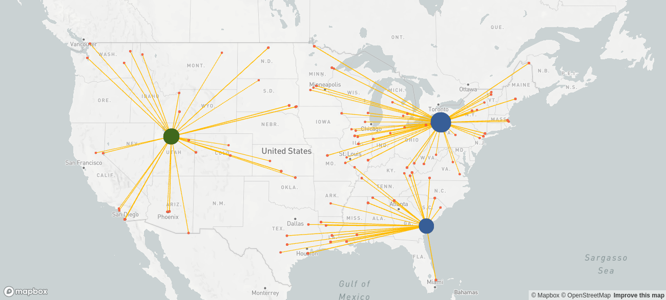
The solution to the baseline scenario could look as follows, where the blue and orange bubbles represent the two existing sites and the customers, respectively, and the volume of each bubble is proportional to its in- or out-flow. The yellow lines indicate the product flow.
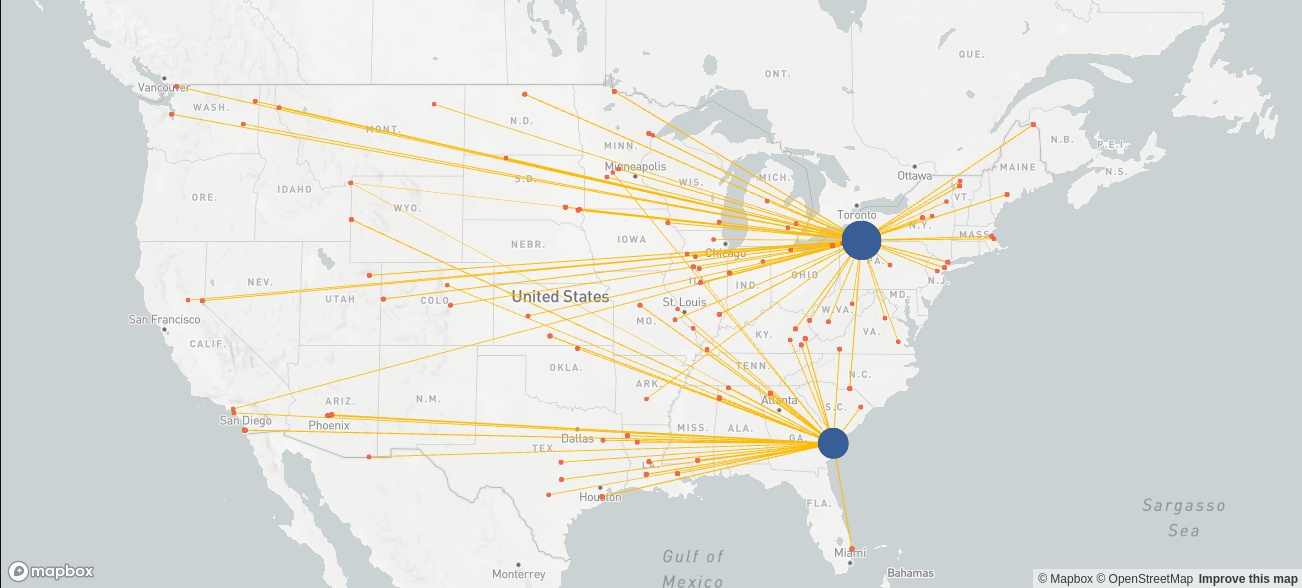
| Total costs | 25,215,399 |
| Fixed costs | 8,833,360 |
| Variable costs | 16,382,039 |
If the above costs match up with the actual costs in that year, we have validated our model.
The optimized baseline scenario
In the map above we can see that some customers are supplied from the site that is actually further away as well as some customers being serviced from both sites. Even before discussing changes to the supply chain network, the management will likely want to know what short-term gains could come from restructuring to eliminate these inefficiencies. That is exactly what is done in the optimized baseline scenario, i.e. we keep the network structure (same sites), but allow the model to optimize the flows. The result looks as follows.
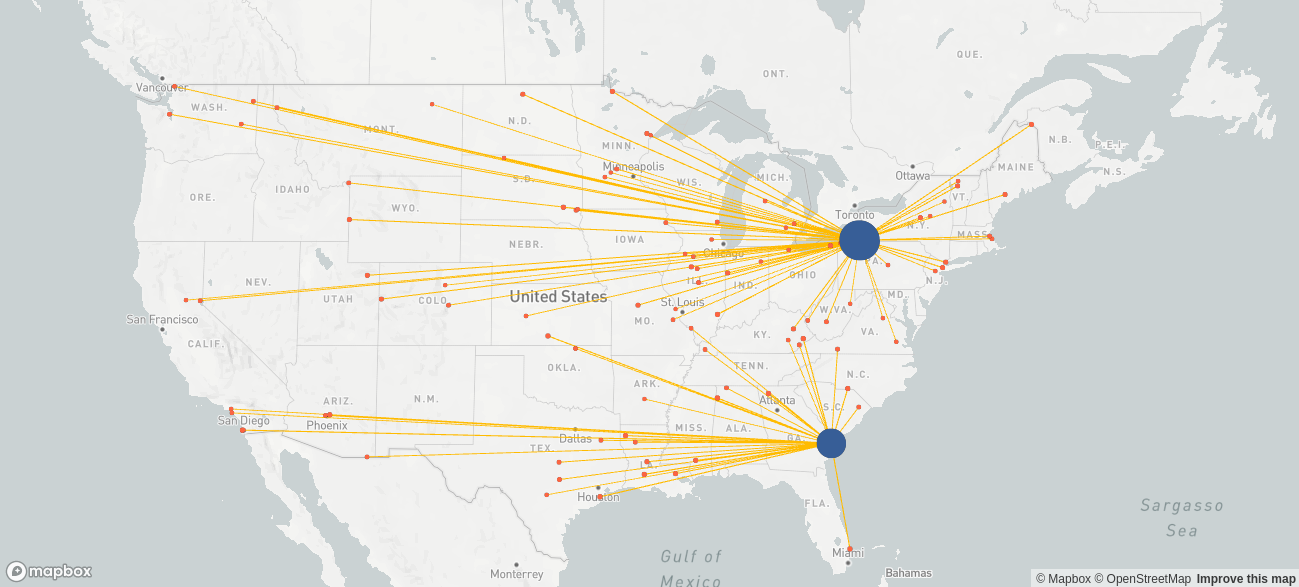
| Total costs | 24,917,771 |
| Fixed costs | 8,833,360 |
| Variable costs | 16,084,411 |
Improving the product flow would reduce the variable costs by up to US$ 300 k (~1.8%).
Future scenarios
So far we have only worked with historical data. From here we would go on to forecast future demand as well as future costs. We might want to consider multiple alternative developments, e.g. one with comparably low and one with higher labor costs. The company expects an increase in demand by a factor of 1.4 across the board, increased fixed costs for the existing sites by a factor of 2 within the next 5 years, and the shipping rates to remain stable.
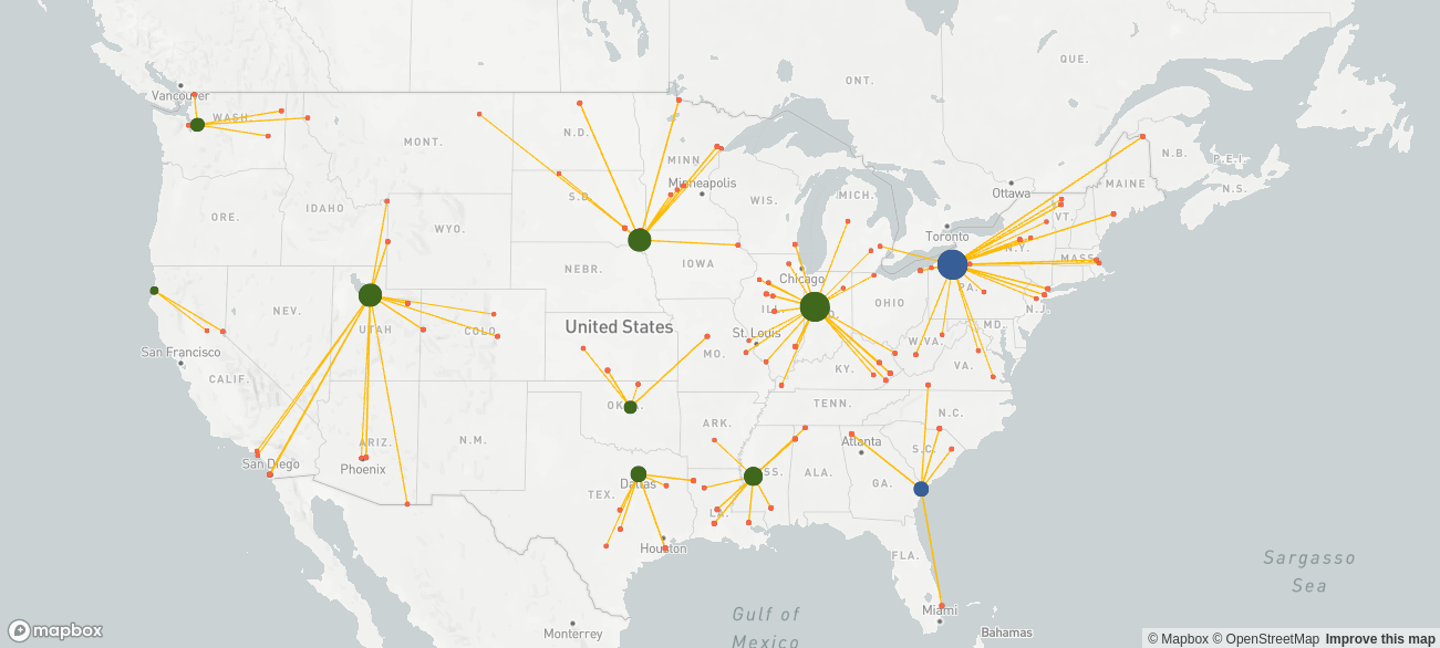
Next, we need to identify potential locations for new warehouses and estimate the fixed cost of the new sites. The company estimates the fixed cost of each new site to be roughly USD 4M per year, and it wants to keep the two warehouses at the east coast. The following map displays the situation, where blue bubbles represent the existing warehouses, the green ones are the potential new locations, and the orange bubbles are the markets.
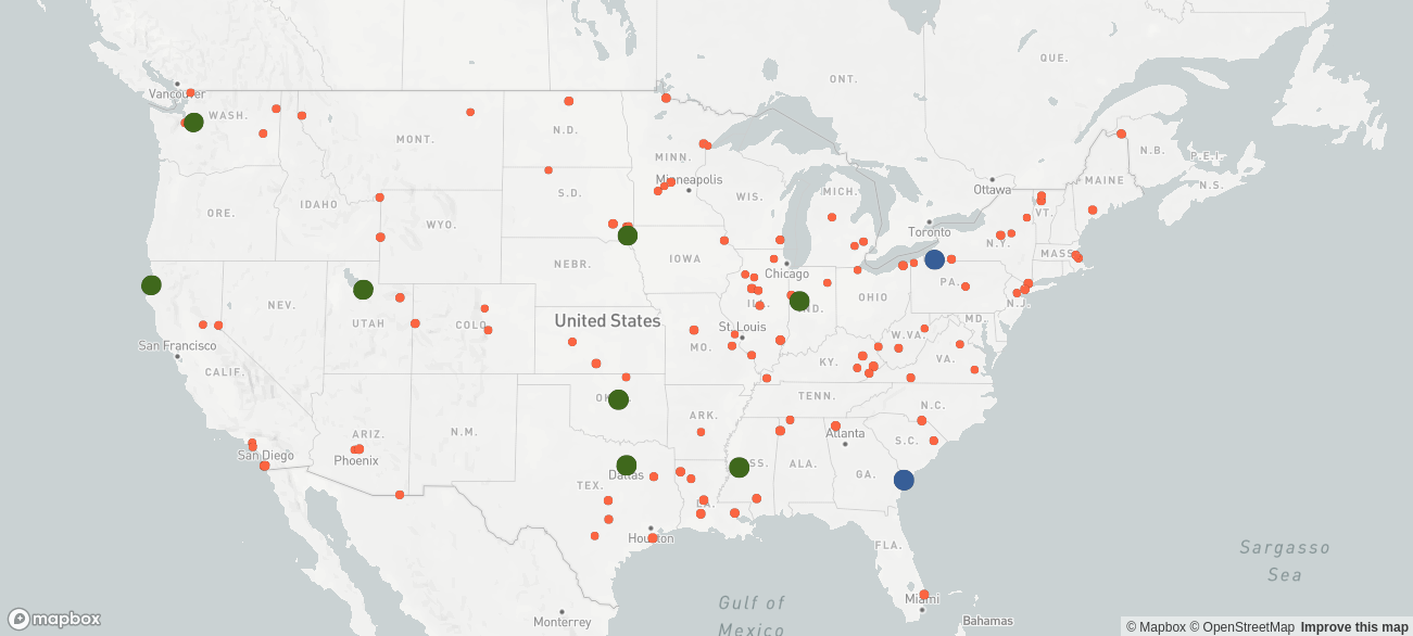
It is common to evaluate multiple possible supply chain network designs in separate scenarios (e.g. a scenario with low capital expenditures, say with at most one new site, a customer-centric scenario with short delivery distances, a scenario where a certain site is included, etc). It is important however to focus on few realistic scenarios.
The cost-optimal future supply chain network design
One particularly interesting scenario is the cost-optimal supply chain network design. In case the management considers choosing an alternative network design, say, one with shorter delivery distances, it can compare this network design against the cost-optimal one to determine the price the company has to pay for reducing delivery distances. To develop the cost-optimal network design, we include only the most essential constraints. The development process is iterative. The initial solutions are often unrealistic, and we need to add constraints until the result is feasible. Given the future circumstances, the cost-optimal network footprint looks as follows.
| Total costs | 24,917,771 |
| Fixed costs | 8,833,360 |
| Variable costs | 16,084,411 |
| Average delivery distance [km] | 806 |
This solution fails in terms of delivery speed, since the distances from warehouses to customers are on average too far.
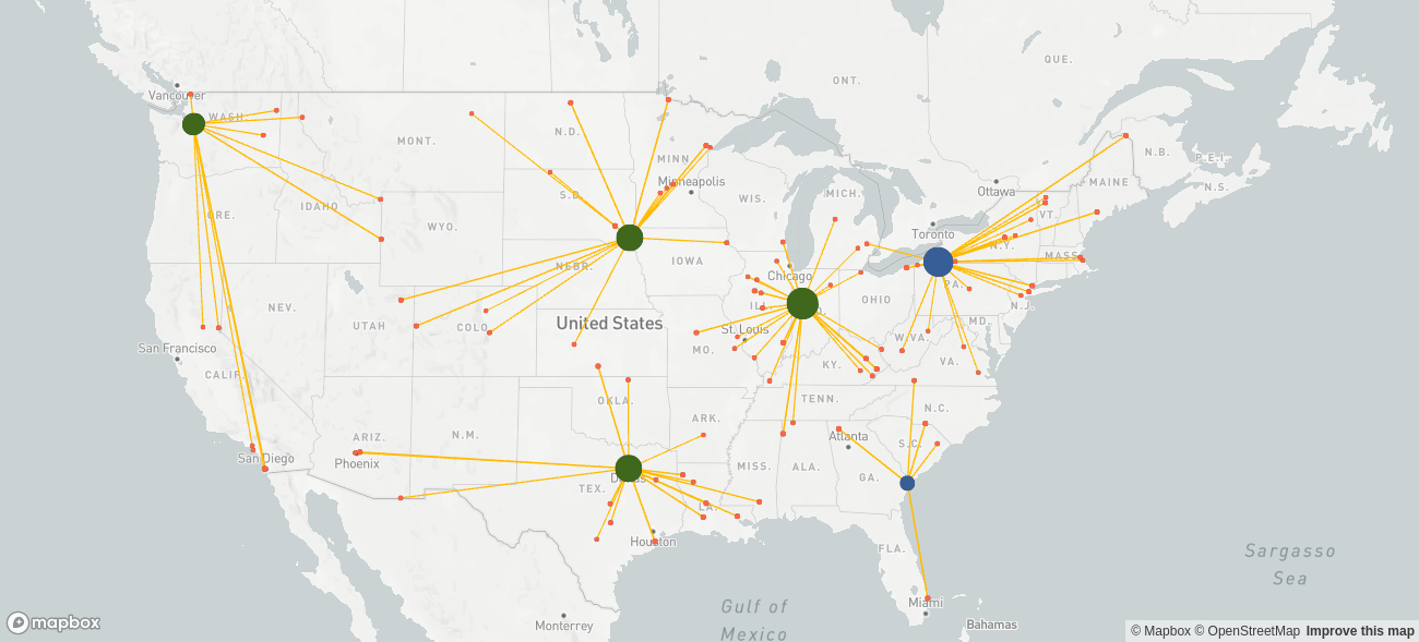
Customer-centric network design
Therefore, we define an additional scenario where we integrate an incentive to avoid deliveries over a distance farther than 500 km, which leads to the installation of more warehouses, and we can see exactly how much more this costs us in comparison to the cost-optimal solution.
| Total costs | 56,722,469 |
| Fixed costs | 49,666,720 |
| Variable costs | 7,055,749 |
| Average delivery distance [km] | 404 |
With this network footprint, fixed costs are significantly higher while variable costs decrease leading to an increase of total costs of 59%. Additionally, this solution requires a lot of capital expenditures. Therefore, it is necessary to modify this scenario.
Balanced scenario
In order to strike a balance between costs and delivery speed, we create multiple scenarios where we set the number of new sites to  . After evaluating each solution, the management agrees that building four new sites best balances costs and delivery speed. The resulting supply chain network looks as follows.
| Total costs | 42,792,873 |
| Fixed costs | 33,666,720 |
| Variable costs | 9,126,153 |
| Average delivery distance [km] | 523 |
The total costs are 20% higher than in the cost-optimal network design, but the average delivery distance is only 523 km compared to 806 km, which aligns with the strategy of the company.
Networks with multiple echelons
The facility location problem is too simple for most practical situations. Let’s see how we can extend this basic model to include additional requirements encountered in real world situations.
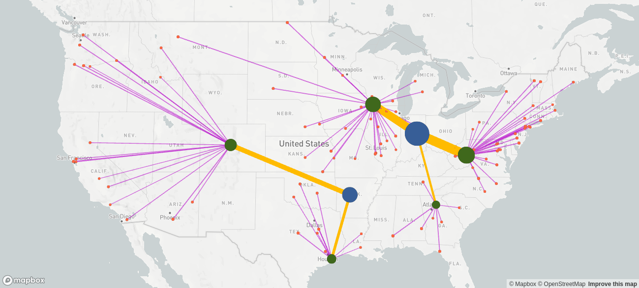
In the facility location problem, product is delivered directly from sites to customers. Such a model is called single-echelon in contrast to a multi-echelon model where product traverses multiple stations. For example, the product could be manufactured in plants from where it is delivered to distribution centers (DCs) from where it is shipped to customers. Typically, the mode of transportation differs depending on source and destination node type, which influences the unit cost. The shipments from plants to DCs are often inter-modal or full truckloads, whereas the shipments from DCs to customers are mostly smaller incurring higher unit costs.
Such a model might generate the following supply chain network design, where the blue / green / orange bubbles are the manufacturing sites / the DCs / the customers, respectively. The yellow connections are the flows from manufacturing sites to DCs, and the purple connections are the flows from the DCs to the customers.
Multiple products
When heterogeneous products share the same network and resources, we need to capture that aspect in the model. It is crucial to find an expedient grouping of individual products into categories which are then used in the model. For example, consider a sports retailer with millions of products. On the one hand, product categories cannot be too broad. For example, products such as rowing machines versus snowboards versus T-shirts must be distinguished since shipping is done differently and demand fluctuates by region. These would require separate categories. On the other hand, product categories should not be too detailed. For example, distinguishing blue and green T-shirts adds little value while making the model more complex. For this example, an appropriate categorization could be: fitness equipment, winter sports equipment, and clothing.
Conclusions
Virtually any supply chain network design model contains the facility location problem. However, there are additional aspects to consider which are specific to the company under consideration, its goals and unique situation. To base strategic decisions on solid ground, it requires adding details to the model which quickly increases the complexity. The complexity in turn increases the development effort, might require trading off accuracy against reduced complexity, and might justify the use of a powerful commercial solver such as CPLEX or Gurobi.
The extensions to the facility location problem shown here are just the tip of the iceberg. Another example is to integrate aspects related to manufacturing to answer questions such as allocation of products to production facilities, if it is necessary to invest in new equipment, and if so, if to opt for specialized and highly efficient equipment or more flexible multi-purpose equipment. In an e-commerce setting, there could be a strong focus on fulfillment, which requires including multiple shipment modes such as same-day, 1-day, and ground shipping options. These examples indicate that it is unlikely that supply chain network design projects in different companies lead to the exact same model.
Furthermore, a network design project is highly dynamic in practice, since insights gained from initially generated solutions lead to further questions and model modifications. When working on a network design project, clarity about strengths and weaknesses of different network designs evolves gradually for all project members. Hence, supply chain network design does involve modeling and implementation, but is, first and foremost, a very interactive process.